Find Markov Steady States Using RREF: Easy Method

A steady-state vector gives the long-run probability of finding a Markov chain in each state. You find it by solving the homogeneous system (P − I)x = 0, then scaling the answer so its entries add to 1. Row reduction (RREF) does the heavy lifting.

Here’s the full method, with a worked example you can reproduce.

What a steady-state vector is

For a Markov chain with transition matrix P, the steady-state (or stationary) vector x satisfies Px = x. Once the chain reaches x, another step leaves it unchanged, so x holds the long-run probability of being in each state.

Two things make x special: it’s an eigenvector of P for the eigenvalue 1, and it’s a probability vector (all entries ≥ 0, summing to 1).

Why the equation is (P − I)x = 0

Start from the fixed-point condition and rearrange:

Px = x → Px − x = 0 → (P − I)x = 0.

That’s a homogeneous linear system. Its solutions form the null space of (P − I), which is exactly the eigenspace for eigenvalue 1. RREF is the fastest hand method for finding that null space.

One convention note that trips people up: this form assumes P is column-stochastic (each column sums to 1, with entry P[i][j] = probability of moving from state j to state i). If your textbook uses a row-stochastic matrix (rows sum to 1, and πP = π), transpose first and solve (Pᵀ − I)x = 0.

Worked example (two states)

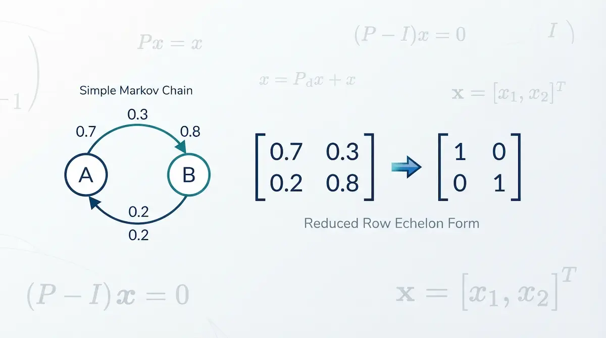
Take a column-stochastic transition matrix:

P = [ 0.9   0.5 ]
    [ 0.1   0.5 ]

Column 1 says: from state A, stay with probability 0.9, move to B with 0.1. Both columns sum to 1.

Subtract the identity:

P − I = [ −0.1    0.5 ]
        [  0.1   −0.5 ]

Now reduce (P − I) to RREF. Scale row 1 by −10, then clear row 2:

[ 1   −5 ]
[ 0    0 ]

The zero row confirms rank 1 and one free variable, which is what a valid steady state needs. Reading the top row:

x₁ − 5x₂ = 0 → x₁ = 5x₂.

Let x₂ = t, so the solution set is x = t(5, 1). Every eigenvector for eigenvalue 1 is a multiple of (5, 1).

Normalize to a probability vector

Scale so the entries sum to 1. Since 5 + 1 = 6:

x = (5/6, 1/6) ≈ (0.833, 0.167).

Check it: Px returns (5/6, 1/6), so the vector is fixed. Long-run, the chain spends about 83.3% of its time in state A and 16.7% in state B.

You can run the reduction on any (P − I) with the RREF calculator and follow the same step-by-step rows.

When a unique steady state exists

A single steady-state distribution is guaranteed when the chain is regular: some power of P has all positive entries (which holds when the chain is irreducible and aperiodic). The Perron–Frobenius theorem then makes eigenvalue 1 simple, so the eigenspace is one-dimensional and the normalized vector is unique.

If (P − I) reduces to more than one free variable, the chain has multiple stationary distributions, usually because it splits into separate communicating classes or contains absorbing states.

Quick reference

• Build P and confirm the stochastic direction (columns vs rows).
• Form (P − I), or (Pᵀ − I) for a row-stochastic P.
• Reduce to RREF and read off the free-variable solution.
• Normalize so the entries sum to 1.

That normalized null-space vector is your long-run prediction.